
Meta-analyses, as I said in the previous part, are methods that allow you to statistically combine the results of different studies. Just as you can calculate the mean height of a group of students by adding up the length of all the students and dividing by the number of students, you can determine the mean effect of studies in a meta-analysis.
To do this, you have to decide on a metric. This metric depends on the outcome parameters that the studies use.
Dichotomous or continuous?
Basically, one has to distinguish between continuous and dichotomous measures. Continuous ones are those that map a continuum. E.g. a scale like a pain scale, a depression scale, or Conners‘ hyperactivity scale, which is a rating scale where different questions are scored and added up at the end, resulting in a continuous score. This is the scale most commonly used in ADHD studies. Blood pressure values, laboratory values and measurements in general, body size, shoe size, temperature, all these are also continuous measures.
To be distinguished from these are the dichotomous measures: dead or alive, sick or healthy, relapsed or not, tall or short, etc.
Effect sizes of studies with dichotomous outcome parameters
For these dichotomous measures, the original studies report prevalence: this many people died in the treatment group, that many in the control group. This is standardized to the total number of patients in each group. The numbers are put into proportion. And you get a measure of the difference between the groups, which is called a relative risk, an odds ratio, a hazard ratio or some other ratio, depending on what exactly is put into the ratio. In these dichotomous outcome measures, a lack of difference between groups is indicated by a ratio of 1. If the outcome number is larger – e.g. 1.5 – then one of the groups is better off by half, i.e. by 50%. Which one that is depends on how the ratio was formed.
Example: Let’s imagine a results table of the following kind:
| Dead | Alive | n | |
| Treatment | 20 | 30 | 50 |
| Control | 30 | 20 | 50 |
| n | 50 | 50 | 100 |
The term “odds” in „odds ratio“ means „chance“, like in a bet, for example. Here, at the top of the table, the chance or odds of dying under the treatment would be 20/30 = 0.66. And the chance of dying under the control treatment would be 30/20 = 1.5. The odds ratio is now the ratio of the two: 0.66/1.5 = 0.44. So a person in the treatment group would have a 44% higher chance of surviving than in the control group.
The relative risk is formed slightly differently: It would be 20/50/30/50, so would relate the events in the two groups to the total number in the group, and would therefore be 0.66.
Standardized mean difference
Continuous measures also form ratios to express the difference between groups. These were the ratios in our meta-analyses. In this case, it is a difference between the results of one group minus those of the other. Again, one has to be careful how the difference is formed. Because, depending on the case, a positive as well as a negative value may express a superiority of the treatment group.
But now we still have to solve the problem that different variables are measured quite differently. Blood pressure and depression scales, for example, have very different metrics. In order to make the difference between the treatment and control group in one study comparable with that of other studies or even with other metrics, we divide the difference by the standard deviation or the spread of the values around the mean. This leads us to obtain a metric expressed in the units of the standard normal distribution or in units of standard deviations (Fig. 1). The standard deviation indicates the spread of the distribution around the mean (for a reasonably normally distributed variable) and has the value „1“ in the standard normal distribution or the Gaussian curve (see the thick line in Fig. 1 below).
Now, if you divide any difference of a continuous variable by its standard deviation, what happens? One standardizes this difference to the standard normal distribution, or expresses the difference in units of standard deviations.
This metric, which only makes sense for continuous values and thus their differences, is called the „standardized mean difference (SMD)“, i.e. the difference between two groups measured with a metric scale. In the end, this SMD is always in the same metric, no matter how large the units were. The abbreviation symbol for this SMD is usually „d“ for „difference“.
We can see: A d = 1 is a difference between two groups that is one standard deviation. So if we were to duplicate the upper curve and shift it to the right or left by the distance of the bold line, the standard deviation, we would have visualized an effect size of d = 1.
An effect size of d = 0.5 is half a standard deviation and already a clinically significant difference. The English authority NICE once demanded times ago that new depression studies should have an effect size of at least half a standard deviation compared to placebo in order to be worth paying for. In fact, the cumulative effect of antidepressants is about d = 0.38, thus much smaller [1].
This, about a third of a standard deviation, is usually the limit below which effects are judged to be „clinically small“. The meta-analysis of psychotherapy studies mentioned earlier revealed a d = 0.6 at that time. This is seen as clinically significant.
If many studies are meta-analysed that also include small studies, then a slightly corrected version of the SMD is used as a metric, which is then called „Hedge’s g“ after Larry Hedges, who invented it. It is slightly smaller because it includes a correction factor that takes into account that smaller studies tend to overestimate the values. But otherwise it’s pretty much the same.
Because a meta-analysis has two groups that often have different standard deviations, a so-called pooled or mixed standard deviation is usually used to calculate it. This is a value where the two standard deviations in both groups are averaged.
Calculating effect sizes for home use
If you want to calculate effect sizes for home use, you can also take the conservative option and use the larger of the two standard deviations for standardization. Anyone can do this using a results table with a pocket calculator. For example, if you see the following values in a results table of a depression study (arbitrary data):
| Before | After | |
| Treatment Group: | 19.5 (4.3) | 16.2 (5.7) |
| Control Group: | 20.1 (4.5) | 18.7 (4.8) |
Then you can calculate the changes, i.e. 3.3 for the treatment group and 1.4 for the control group. Or, to make it even simpler: you can simply use the values at the end of the treatment, because we assume that due to randomization, i.e. random allocation, the initial values in both groups only fluctuate randomly and can therefore be ignored. The difference between the two groups at the end of the treatment would be 2.5. Now either use the larger standard deviation of the two, i.e. 5.7 for standardization, or average the two values in brackets, i.e. 5.25. If we divide 2.5 by 5.7, we get d = 0.44, i.e. a difference of 0.44 standard deviations between the groups. If we were to use the difference values, i.e. 1.9 and divide by the averaged standard deviation, the effect would be smaller, d = 0.38.
As you can see, it is very easy to calculate effect sizes for individual studies using this method to get an idea of the clinical significance of the reported effect.
Caution: Sometimes tables of results in studies do not report the standard deviation (SD), but the standard error of the mean (SEM). This is a value that indicates the statistical variation in the estimate of the mean. While the standard deviation is the estimate of a distribution value and only has something to do with the size of the study insofar as larger studies provide this estimate more precisely, the standard error of the mean is directly dependent on the size of the study, namely via the relationship SEM = SD/root of n. It can thus be seen directly: the larger the number of study participants n in a study, the smaller the standard error, i.e. the estimation error of the mean. However, because the standard deviation is included in this formula, it can be calculated back if only SEM is given by reformulating the formula arithmetically. Then you get SD = SEM * root of n.
Summarizing effect sizes
In a meta-analysis, an effect size measure is formed for each study as a difference measure d or g between the treatment and control group, or a ratio measure if you are dealing with dichotomous values. If a study has several outcome parameters, one can either take only the main outcome criteria. Or one averages the effect sizes at study level, or, for example, if similar outcome measures are available across several studies, then one calculates a separate analysis for each of the different outcomes. This depends very much on the situation and the goal of the analysis. This goal and the methodology used must be considered in advance and formulated in a protocol, which ideally should also be registered in a database or otherwise published in advance. Then readers of the meta-analysis can check whether you have adhered to your own guidelines, and you protect yourself from „generating“ results by trial and error that actually represent a random variation. The corresponding database for systematic reviews and meta-analyses is called „PROSPERO„.
Now, if you have an effect size measure d/g or a ratio (odds ratio, risk ratio, etc.) for each study, you have to combine them for a meta-analysis.
In principle, it works like this: You calculate a mean value, similar to the way you calculate the mean height of a class of children. This automatically gives you a scatter value, i.e. a measure of how much these individual effect sizes scatter around the mean. If we take my Fig. 4 from the article on our ADHD meta analysis, we see: The individual effect sizes scatter very strongly around the mean value of approx. g = 0.2.
Such a situation is described as heterogeneous, and one usually assumes that there are influences that one does not know about that cause this scatter. Therefore, in order to summarize such heterogeneous effect sizes, a statistical model is used which assumes that there is not only a true mean value and an unknown error deviation from it, but a true mean value, an unknown error deviation and a scatter term behind which there are systematic influencing variables. This is estimated. In this case, one assumes a so-called „random effects“ model, otherwise it is a simpler „fixed effects“ model.
By determining the dispersion, one can also make a significance calculation. This tells us whether an effect size found is statistically super randomly different from zero, completely independent of the effect size.
There are meta-analyses that find very small effects that are significant (e.g. because all effects are very homogeneous, because the studies are large and have examined many patients). There are meta-analyses that isolate very large effects, but these are not significant (e.g. because there are only a few, small studies that are highly scattered).
Therefore, one must always look at the absolute size of the effect, not only at the significance.
The result of a meta-analysis is then presented in a so-called forest plot or tree graph. I reprint here our meta-analysis of the Arnica trials (Fig. 2).

Each line is a study. The metric is Hedge’s g, which is a variant of the standardized mean difference; next to it are the ratios (standard error and variance) needed to calculate the significance of the effect size, or the 95% confidence interval. If this confidence interval does not include the zero limit for both the individual studies and the summary, then an individual study or the overall value is significant.
We see for example: Most studies cluster around the mean of g = 0.18, which the random effects analysis calculates as the common mean. One study, Brinkhaus et al 3, is completely out of the ordinary: It has a huge effect size of g = 2 and does not fit into the graph scheme at all. Some studies are even negative. These are the ones that also land below the zero line in Fig. 4 from the article on our ADHD meta analysis. Only Pinsent’s study is individually significant, because here the 95% confidence intervals do not intersect the zero line.
The diamond indicates the joint value of the mean effect size. The rhombus touches the zero line very slightly because the error probability of p = 0.059 is slightly above the conventional significance threshold of 5%. One can see from the p-value in the last column that the statistical summary value of a fixed effects analysis is quite significant. But you can see from the heterogeneity measure, in this case the I2, which quantifies the extent of dispersion and is significant, that a fixed effects analysis is out of place.
So you can see from such a forest plot both the individual effect sizes, as well as their dispersion and the summary effect size in the rhombus. The distance of the rhombus from the zero line shows how large the effect is. The thickness of the rhombus, and whether it overlaps the zero line or not, shows how strongly this summary effect is or is not different from zero.
As an example of a meta-analysis that summarized dichotomous measures, consider the analysis by Drouin-Chartier and colleagues [3]. They investigated the effect of egg consumption on mortality. The analysis is shown in Fig. 3. These were cohort studies, i.e. observational studies on two groups, some of which compared people who eat eggs with those who do not, over very long periods of time. The background is the notorious cholesterol hypothesis of coronary heart disease. Supposedly, the cholesterol in eggs is dangerous. This was investigated in these cohort studies: over 32 years, with more than 5.5 million man-years. You can see from the sum statistics, the effect measure „relative risk“: this is RR = 0.98, i.e. slightly below 1. This means: egg-eating people even have a slightly lower risk of dying from heart disease. But the effect is not significant because the confidence interval includes 1, the line of equality or no effect. You can tell by the weight which studies were larger; because those are more heavily weighted.
So after 32 years and many millions of research dollars, we know what we always suspected: Eggs are not harmful. But now we really know. You can see: The principle and the presentation is the same as in the analysis above. Only the metric is different because the target criterion of the studies was different, namely a dichotomous one, e.g. stroke or not, heart attack or not, dead or not.

Fig. 3 – Meta-analysis of studies that investigated the impact of egg consumption on mortality, from [2].
Sensitivity analyses
Meta-analyses have several aims. One is to calculate a common effect size of different studies and find out whether it is significantly different from zero, i.e. statistically significant. Another is to quantify the effect, i.e. to see how big it is. A statistically significant effect of d = 0.2 is usually not very interesting clinically. An effect of d = 1.0, even if it is not statistically significant, can still be significant because it might mean that you have to do another study or two to confirm it.
But often it is more interesting to find out what actually causes the scatter in effect sizes. This is done with sensitivity analyses. Studies are often different: they have different durations, different populations, different study designs and outcome measures. However, studies can be analysed separately according to these differences, and it can be determined whether the heterogeneity decreases as a result. Then one knows the drivers of this dispersion.
If a possible moderator variable is continuous, then one can examine this variable within the framework of a regression analysis. Here, as briefly described above, the moderator variable, for example the year of publication of a study, is used to predict the effect size. If the variable has an influence, the result is a significant model.
As an example of a significant regression model in the context of a meta-analysis, I show here below in Figure 4 a meta-regression from our meta-analysis of studies on mindfulness interventions with children in schools [4]. The analysis yielded an overall significant effect size of g = 0.4, and even g = 0.8 for cognitive measures. However, the heterogeneity was very large. It could be clarified by a regression of meditation intensity on effect size (Figure 4):
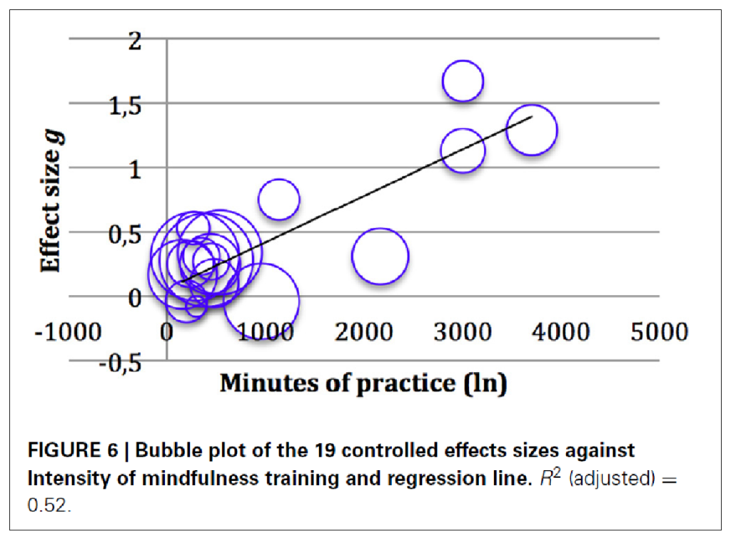
We thus know: The longer (in trend) the children meditated, the larger the effect in the study. The size of the bubbles indicates the size of the studies. On the left, on the y-axis, the effect size is plotted. Below, on the x-axis, the duration of the practice. One can see in the tendency that the effect sizes increase the longer the practice duration was. Of course, there are also outliers: a study with very high effects and short practice, and one with longer duration and still small effects. But in the tendency one recognizes an increase.
Such sensitivity analyses help to find out what needs to be taken into account in further studies. In this case, one would assume that it is useful to increase the duration of practice if one wants to see larger effects.
In our ADHD meta-analysis, we saw that the biggest effect came from a study that lasted over a year. So in another study, you would try to increase the duration of treatment.
You can also use sensitivity analyses to see how vulnerable the analysis is to assumptions. Then you would remove studies with a certain design. Or, for non-significant analyses, you could calculate how many more studies of that size would be needed to get significant effects. Or you could break down the studies according to different types of interventions. It all depends on the research question and the researcher’s interest.
Meta-analyses are snapshots
Meta-analyses are not meant to last. You can prove with a clever photograph that horses can fly: if you press the shutter release just at the moment when the horse has all four legs in the air while galloping. Horses can’t fly, of course. It is similar with meta-analyses. If you take all the studies together at a certain point in time, there could well be a significant – or non-significant – effect. If another well-done study is added, the picture can change again.
This is why caution is needed with older analyses. And that is why extra caution is needed especially with those meta-analyses in which not really all studies are included. Often, studies with negative results are not published. This of course distorts the picture. Therefore, it is important to check the search strategy for published meta-analyses. Are non-published studies also included? Is the grey literature – theses, doctoral dissertations, academic theses, in which „bad“ results are often hidden – also covered?
You can achieve this full coverage by contacting researchers in the field, writing to companies, etc. In the case of drug studies, it is now also quite common to ask for the documents of the regulatory authorities. Peter Doshi, Peter Gøtzsche and colleagues achieved this at the EMA, the European regulatory authority [5]. But this means thousands of pages of paper coming your way.
Therefore, when reading meta-analyses, it is not only important to look at the results, but also at how the literature search was conducted.
In any case, meta-analyses are useful for summarizing the state of a discipline. In the case of our homeopathy analyses, you can see that: Sometimes homeopathy is effective and sometimes even better than placebo. In any case that is true for ADHD.
Quellen und Literatur
- Turner EH, Matthews AM, Linardatos E, Tell RA, Rosenthal R. Selective publication of antidepressant trials and its influence on apparent efficacy. New England Journal of Medicine. 2008;358:252-60.
- Gaertner K, Baumgartner S, Walach H. Is homeopathic arnica effective for postoperative recovery? A meta-analysis of placebo-controlled and active comparator trials. Frontiers in Surgery. 2021;8:680930. doi: https://doi.org/10.3389/fsurg.2021.680930
- Drouin-Chartier J-P, Chen S, Li Y, et al. Egg consumption and risk of cardiovascular disease: three large prospective US cohort studies, systematic review, and updated meta-analysis. BMJ. 2020;368:m513. doi: https://doi.org/10.1136/bmj.m513
- Zenner C, Herrnleben-Kurz S, Walach H. Mindfulness-based interventions in schools – a systematic review and meta-analysis. Frontiers in Psychology. 2014;5:art 603; doi: https://doi.org/10.3389/fpsyg.2014.00603
- Doshi P, Jefferson T. The first 2 years of the European Medicines Agency’s policy on access to documents: secret no longer. Archives of Internal Medicine. 2013;doi: https://doi.org/10.1001/jamainternmed.2013.3838.